14C Calibration the Bayesian way
Appetizer
With what follows I want to demonstrate that the basic functionality of Oxcal is reflected in this tiny bit of code:
calf<-approxfun(intcal13[,1],intcal13[,2])

likelihood <- function(proposal){dnorm(calf(proposal),bp,std)}

#Setup
collector <- bp <- 3600; std <- 30; last_prob <- likelihood(bp)

for (i in 1:10000) {
  proposal <- rnorm(1, tail(collector,1), 3*std)
  proposal_prob <- likelihood(proposal)

  if ((proposal_prob/last_prob) > runif(1))
  {
    last_prob <- proposal_prob
  } else {
    proposal <- tail(collector,1)
  }

  collector <- c(collector, proposal)
}
Motivation
The ¹⁴C cycle
¹⁴C is produced in the atmosphere by solar radiation, is than oxidised to CO2 and than introduced into the foodchain. From than onward, the ¹⁴C decays.
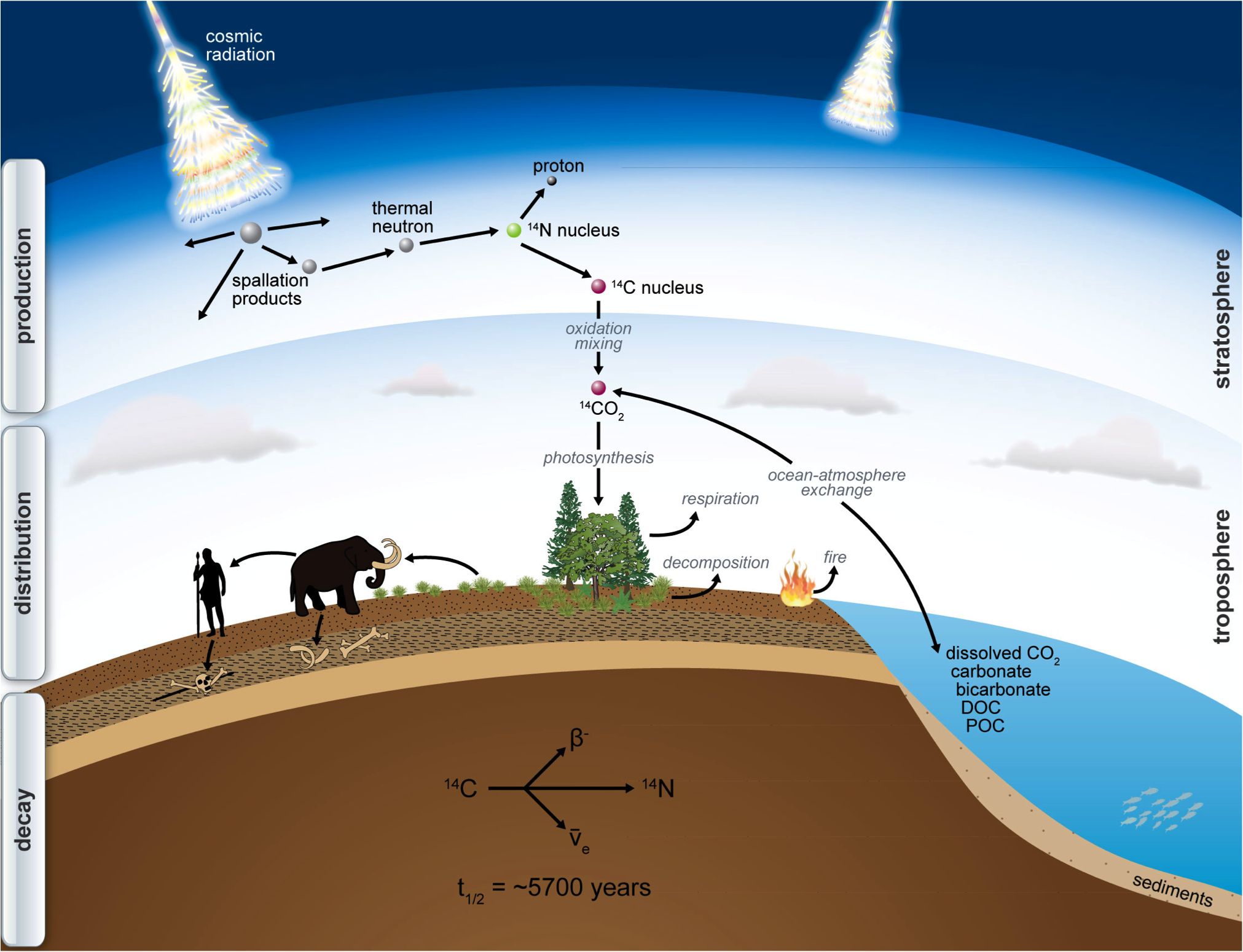
source: http://www.imprs-gbgc.de/uploads/RadiocarbonSchool/Overview/radiocarbon.png
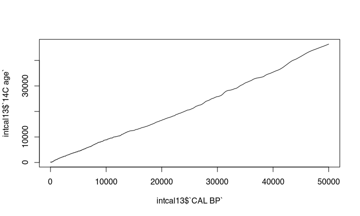
The nonlinear nature of the ¹⁴C curve
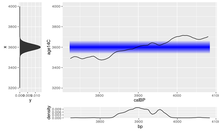
The problem is, that the amount of ¹⁴C in the atmosphere was different during different times. This causes that there is no simple linear relationship between ¹⁴C years you get from the lab to the real calendric cal bp or bc date. The expression of this is the wiggly nature of the calibration curve:
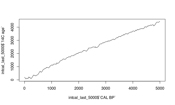
This becomes more obvious if we zoom in:
changes in solar activity
The main reason for that might be the fluctuation of the solar activity, that causes different amount of solar radiation and with that also different ¹⁴C values. One fluctuation is a well known 11 year cycle, but there are other, not so well behaving fluctuations, too.
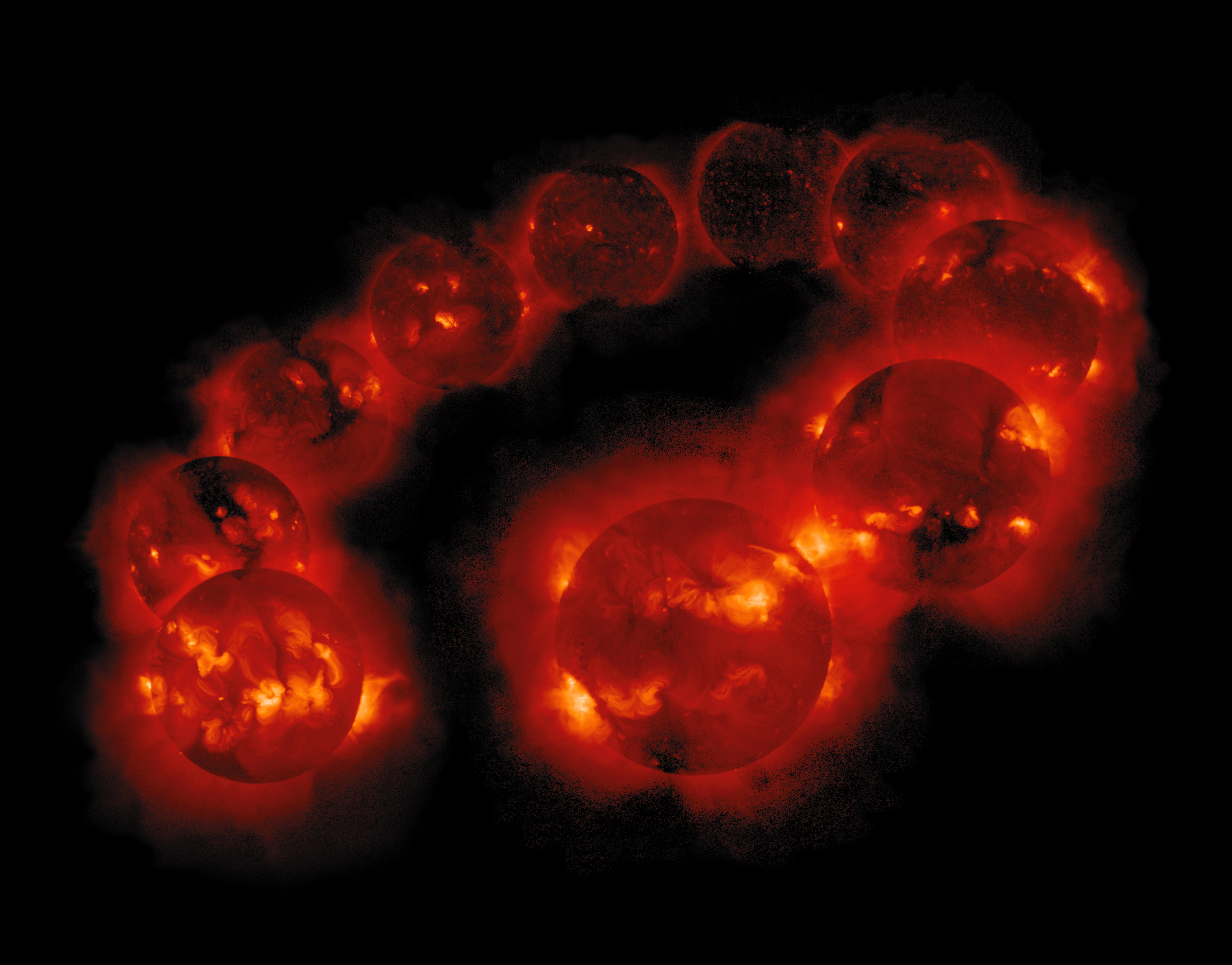
A solar cycle
source: https://upload.wikimedia.org/wikipedia/commons/c/c2/The_Solar_Cycle_XRay_hi.jpg
calibration | using material of known age
To cope with that, we use samples of known age, eg. tree rings. Radiometric dating those gives us a estimation for the amount of ¹⁴C at different times. Since the resulting calibration curve is not linear, there is no linear calculation possible to come up with the real age of things.
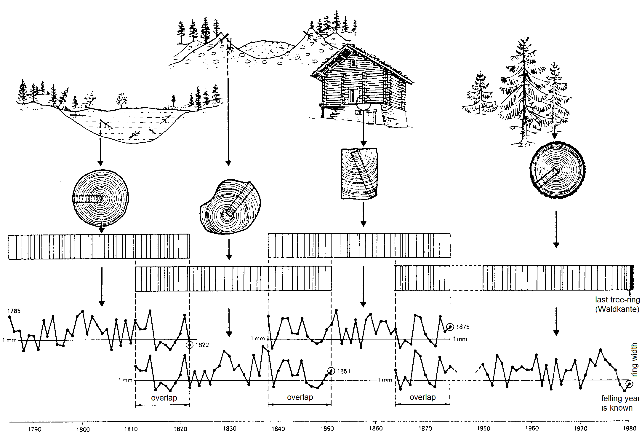
Dendrochronology
source: Schweingruber, F.H., 1983: Der Jahrring. Haupt, Bern und Stuttgart
Real world calibration | The problem with the nonlinear nature
In an ideal world, you could use a ruler for translating a radiocarbon age to a calender age. But due to the wiggles of the curve, there are parts where a radiocarbon age could result in two or even more possible calendric ages.
Real world calibration | The problem nature of a ¹⁴C date
What makes things worse, is the fact, that you will never get a single radiocarbon age, but always a probability distribution with a ‘most likely’ value (the uncalibrated ¹⁴C age) with a standard deviation (eg. +/- 25). On the pro side is that this distribution behaves statistically well, since it follows a normal distribution. On the con side: this enlarges the possible range where a calibration gives multiple values, and it makes the calculation non-trivial.
There are several approaches for calibration, one I have shown in an earlier post, this time we will deal with the Bayesian way.
The bayesian approach to that problem
Keywords
There are several buzzwords that show up when people talk about Bayesian calibration. Those are eg.
- Monte Carlo
- Markov Chain
- Metropolis–Hastings algorithm
The sound impressive, don’t they. But we will handle them one by one.
Monte Carlo
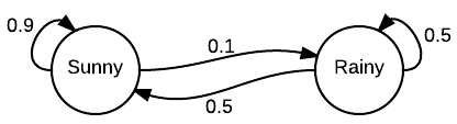
Markov Chain
Together it is MCMC
MCMC stands for ‘Monte Carlo Markov Chain’. This is a procedure that can be used for estimating parameter that can not be measured directly, based on an external evaluation.
To demonstrate that and to prepare for the real ¹⁴C calibration, we will estimate the value of Pi.
Excurse Value of Pi using MCMC
Setting
We have a square of 1 m and an circle with radius 1 m.
We throw darts. We count, how many darts are in the circle, and how many are in the surrounding square.
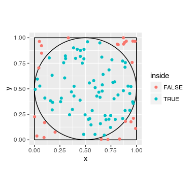
The darts are the random part (Monte Carlo). The amount of darts inside the circle is relative to the area, as it is the amount of darts within the square.
area of circle to area of square is:
\(\frac{\text{area of circle}}{\text{area of square}} = \frac{ r^{2} \cdot \pi }{ (2 \cdot r)^{2} } = \frac{ \pi }{ 4 } = \frac{\text{darts in circle}}{\text{darts in square}} = P\)
\(\pi = P \cdot 4\)
To calculate the value of Pi, we have to count the darts that are inside the circle and those inside the square, and divide their ratio by 4.
Experiment
Now some R code follows:
We make a circle with radius of 0.5 and center it in a square (center = 0.5;0.5). We make a loop, that is repeated 10000 times. We randomly draw from a uniform distribution x and y for the point (we throw the dart). We check if the dart is inside the circle. If so, we memorize it. Afterwards, we divide the amounts of dart inside the circle by the number of trials, divided by 4.
radius <- 0.5
center_x <- center_y <- 0.5
collector <- vector()
for (i in 1:10000) {
x <- runif(1)
y <- runif(1)
inside <- (x-center_x)^2 + (y - center_y)^2 < radius^2
collector <- c(collector,inside)
}

sum(collector==TRUE)/length(collector)*4
The result:
## [1] 3.1208
is close to Pi:
pi
## [1] 3.141593
Experiment Live
Here you can see the experiment running live:
Anatomy of the algorithm
The algorithm we have used can be divided into several parts:
# Setup
radius <- 0.5
center_x <- center_y <- 0.5
collector <- vector()

# Loop
for (i in 1:10000) {

  # Proposal (function)
  x <- runif(1)
  y <- runif(1)

  # Likelihood (function)
  inside <- (x-center_x)^2 + (y - center_y)^2 < radius^2

  collector <- c(collector,inside)
}
- A setup, where we define start values
- A loop, within which things are repeated for some time
- A proposal function, that proposes candidates for our ‘desired’ result (darts in the circle).
- A likelihood function that determinates how likely it is that we archived a ‘desired’ result. In this case it is either in or out, so likelihood is either 0 or 1.
- At last, a collector, that collects our results.
Pi vs ¹⁴C Date
In this experiment, there are already several aspects that are similar to the ¹⁴C calibration that we intend to produce, but also some differences that we have to cope with:
| Pi | ¹⁴C Date |
|---|---|
| unknown value of Pi | unknown distribution of calibrated date |
| choosing a random point | choosing a random date |
| evaluation against the circle (inside/outside) | evaluation against the uncalibrated date |
| deterministic evaluation criterion (inside/outside) | probabalistic criterion (prob. distribution of uncalibrated date) |
With some little effort we will be able to proceed from here to Bayesian calibration.
Toward the Bayesian calibration
Lets start with things that are similar:
Setup
Setup looks rather similar. We only need different things, like uncalibrated date and its standard deviation.
# Pi
radius <- 0.5
center_x <- center_y <- 0.5
collector <- vector()
# Calibration
bp <- 3600
std <- 30
collector <- vector()
collector[1] <- bp
Loop
Also the loop is rather similar:
# Pi
for (i in 1:10000) {
  # Actions that are repeated
  # 10000 times
}
# Calibration
for (i in 1:10000) {
  # Actions that are repeated
  # 10000 times
}
Proposal function
In case of Pi, we propose random x and y coordinates. For the calibration, we propose a calendric date. But we do not propose any random date, but one that depends on our previous proposal. This is a Markov Chain, remember? We make a new proposal near to our previous one, and we make it more likely that it is nearer than that it is farther away. For that we use a normal distribution (rnorm).
# Pi

x <- runif(1)
y <- runif(1)
# Calibration
proposal <- rnorm(
  1,
  tail(collector,1),
  3*std)
Putting together what we have now:
bp <- 3600
std <- 30
collector <- vector()
collector[1] <- bp

for (i in 1:10000) {
  proposal <- rnorm(1, tail(collector,1), 3*std)

  # What is missing is the likelihood function!

  collector <- c(collector, proposal)
}
Differences to the Pi example
From now on, things are a bit different due to the differences of our examples:
| Pi | ¹⁴C Date |
|---|---|
| unknown value of Pi | unknown distribution of calibrated date |
| choosing a random point | choosing a random date |
| evaluation against the circle (inside/outside) | evaluation against the uncalibrated date |
| deterministic evaluation criterion (inside/outside) | probabalistic criterion (prob. distribution of uncalibrated date) |
We cannot directly evaluate, if the date fits our calibrated date, because we do not know it yet. But we know the uncalibrated date, and will use that instead. Also, we do not have a inside/outside of the circle criterion (0/1), but one that has a certain probability, so values between 0 and 1 are possible. We will cope with that.
Differences to the Pi example
Problem One
We evaluate against the uncalibrated date:
-> We have to backcalibrate the proposal
Problem Two
We have a probabilistic criterion, we only get a probability back if the proposal fits our uncalibrated date
-> We have to introduce some probabilistic (random) decision
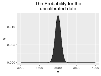
Solution One: Backward calibration
In contrast to forward calibration, backward calibration is straight forward. We can use the ‘ruler approach’, since every calibrated date only reflects one uncalibrated one. The wiggles only go up and down, luckily not left and right!
intcal13 <- read.csv(
  "http://www.radiocarbon.org/IntCal13%20files/intcal13.14c",
  skip = 11, header=F)[,1:2]
colnames(intcal13) <- c("CAL BP", "14C age")

calf <- function(this_bp) {
  approx(intcal13$`CAL BP`,
         intcal13$`14C age`,
         this_bp)$y
}
calf(3600)
## [1] 3364
Likelihood function
For the likelyhood function, we need the shape of the uncalibrated date. With that we can now check how good a proposed date would fit our uncalibrated one. We can determine, how likely a proposal would be given our uncalibrated date.
likelihood <- function(proposal){
 pred = calf(proposal)
 dnorm(pred,bp,std)
}

likelihood(3600)
## [1] 4.85012e-16
With that, we have a likelihood function!
Solution Two: Evaluation with a random component
- We take the last proposal, resp. its likelihood
- We compute the likelihood of the new proposal
- If the new proposal fits better to the uncalibrated date, we keep it
- If not: We still keep it with a probability equal to how worse the new proposal is compared to the prior one
p(new)/p(old)
-> Metropolis-Hastings algorithm
Solution Two: Evaluation with a random component
We start with the bp value of the uncalibrated date as our first proposal. Than we make a second proposal, in relation to the first one.
first_proposal <- bp
second_proposal <- rnorm(1, first_proposal, 3*std)
second_proposal
Our second proposal is:
## [1] 3555.349
With our likelihood function, we check how likely this second proposal is:
ratio <- likelihood(second_proposal)/likelihood(first_proposal)
ratio

## [1] 3.353998e-10
The second proposal is 3.3539984 * 10-10 times likely compared to the first.
Solution Two: Evaluation with a random component
If the ratio is more than 1 (second proposal is better), we keep it.
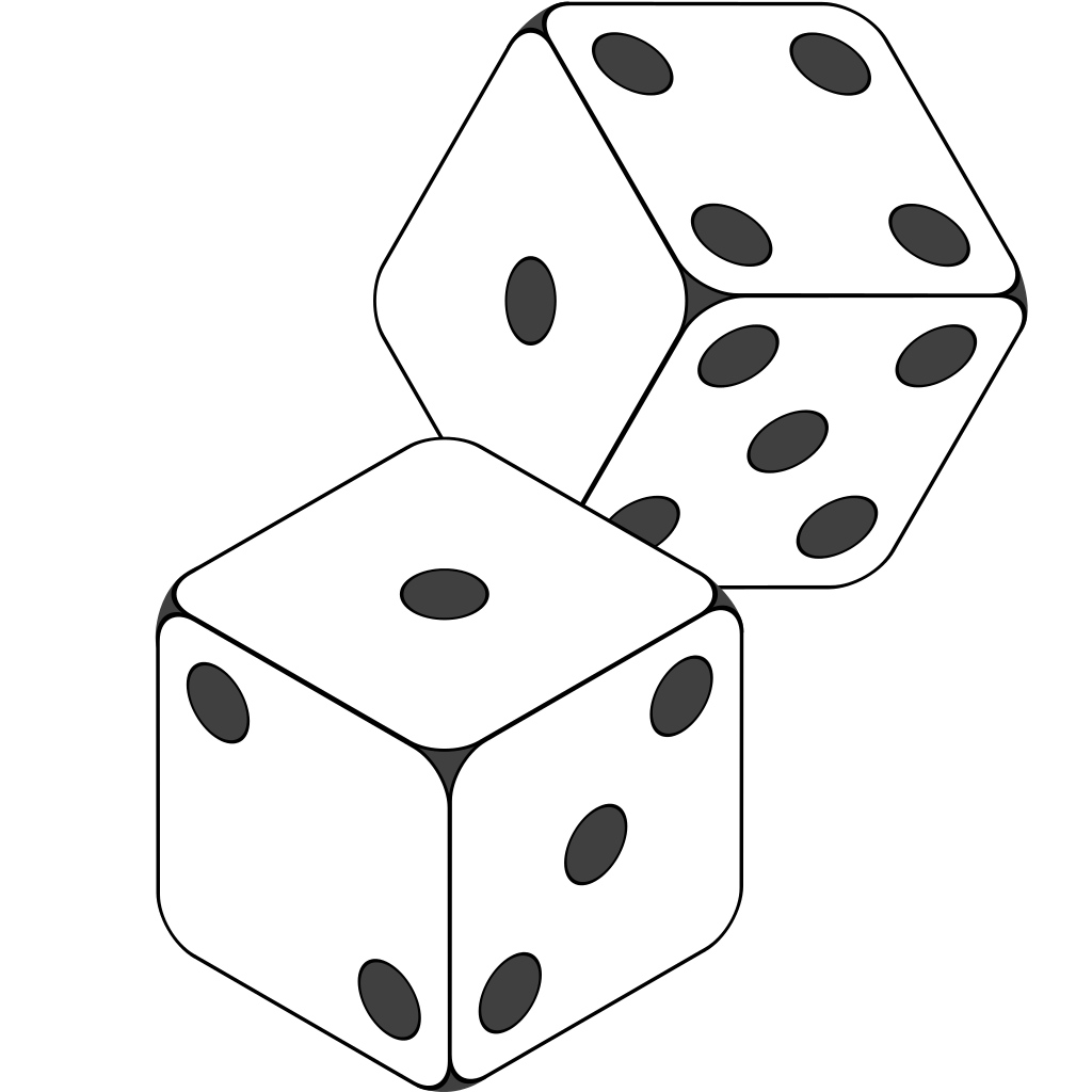
If it is less than one (second proposal is worse), we keep it with a probability equal to the ratio. Meaning, we roll a dice…
alpha <- runif(1)
alpha

## [1] 0.2552167
Check if our random value is smaller than our ratio.
alpha < ratio

## [1] FALSE
That is false. So our second proposal will not be recorded, and will not be part of the Markov chain.
Everything together
The final code
calf<-approxfun(intcal13[,1],intcal13[,2])

likelihood <- function(proposal){dnorm(calf(proposal),bp,std)}

#Setup
collector <- bp <- 3600; std <- 30; last_prob <- likelihood(bp)

for (i in 1:10000) {
  proposal <- rnorm(1, tail(collector,1), 3*std)
  proposal_prob <- likelihood(proposal)

  if ((proposal_prob/last_prob) > runif(1))
  {
    last_prob <- proposal_prob
  } else {
    proposal <- tail(collector,1)
  }

  collector <- c(collector, proposal)
}
With every loop, our collector records those proposals that were accepted, either because they were better, or because the were choosen in the relegation round… due to the random factor.
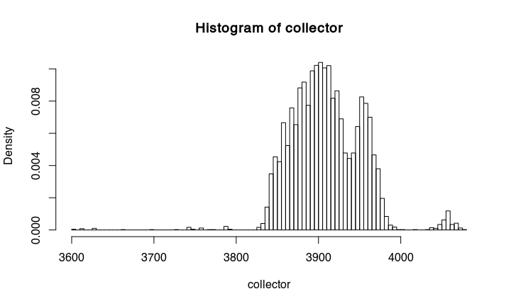
The result
If we make a histogramm from the collected proposals, we get something that is essentially already the calibrated date:
hist(collector,probability=TRUE, breaks = 100)
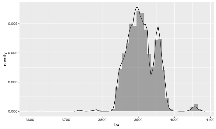
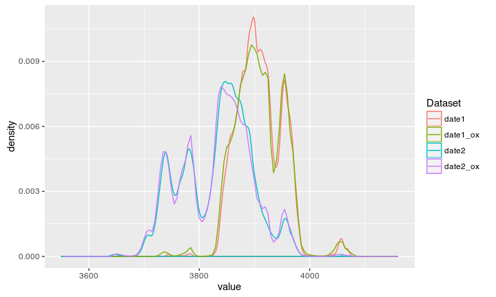
Compare the result
We can compare the resulting histogram with a calibration from Oxcal: looks similar!
See it run
Adding stratigraphical informations
The Scenario
We have two samples, S_1 (3600, 30) and S_2 (3550, 40). We know from the stratigraphy, that S_1 must be younger than S_2.
We can easily introduce this information into our calibration with a little extra code.
The new code
First step: Calibrate multiple dates at once. For this, we add another dimension to our variables (bp, std, collector, last_prob), to reflect the fact that we now deal with multiple data:
#Setup
bp <- c(3600, 3550); std <- c(30,40)
collector <- list(date1=bp[1], date2=bp[2])
last_prob <- c(likelihood(bp[1]), likelihood(bp[2]))

for (i in 1:20000) {
  curr_date <- (i-1)%%2+1 # alter between 1 and 2
  proposal <- rnorm(1, tail(collector[[curr_date]],1), 3*std[curr_date])
  proposal_prob <- likelihood(proposal)[curr_date]

  if ((proposal_prob/last_prob[curr_date]) > runif(1))
  {
    last_prob[curr_date] <- proposal_prob
  } else {
    proposal <- tail(collector[[curr_date]],1)
  }

  collector[[curr_date]] <- c(collector[[curr_date]], proposal)
}
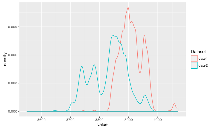
The result
If we now let the code run, we can calibrate two dates at once:
The new code
Second step: Alter the Metropolis-Hastings -> Gibbs Sampling We add another condition:
If calibrating for the first date (S_1), every proposal must be younger than the last proposal for the second date (S_2), and vice versa,
If calibrating for the second date (S_2), every proposal must be older than the last proposal for the second date (S_1)
#Setup
bp <- c(3600, 3550); std <- c(30,40)
collector <- list(date1=bp[1], date2=bp[2])
last_prob <- c(likelihood(bp[1]), likelihood(bp[2]))

for (i in 1:20000) {
  curr_date <- (i-1)%%2+1 # alter between 1 and 2
  proposal <- rnorm(1, tail(collector[[curr_date]],1), 3*std[curr_date])
  proposal_prob <- likelihood(proposal)[curr_date]

# This is the new bit!
#####################################################
  if (curr_date == 1 & proposal > tail(collector[[2]],1)) proposal_prob = 0
  if (curr_date == 2 & proposal < tail(collector[[1]],1)) proposal_prob = 0
#####################################################

  if ((proposal_prob/last_prob[curr_date]) > runif(1))
  {
    last_prob[curr_date] <- proposal_prob
  } else {
    proposal <- tail(collector[[curr_date]],1)
  }

  collector[[curr_date]] <- c(collector[[curr_date]], proposal)
}
The result
Now we can see the modeled date according to our stratigraphic information:
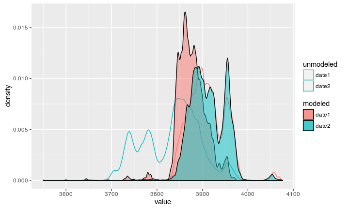
Both dates can again be compared against the Oxcal output:
Compare to Oxcal unmodeled
Compare to Oxcal modeled
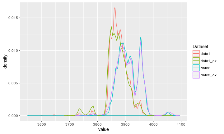
Result
Voila, Oxcal reverse engineered!