14C Calibration 1
Calibration of 14C dates is one of the more common tasks an archaeologists has to do. I will not go into the details of the details why calibration is necessary here (maybe in another post), but I want to give in this post and in some follow ups hands on instruction how a calibration can be archieved using R. This series will be published also at the ISAAKiel-Repository.
The short story
Everything, what follows, is an explanation of these 5 lines of code:
cal_curve <- read.csv(
url("http://www.radiocarbon.org/IntCal13%20files/intcal13.14c"),
skip=11,
header=F)
cal_matrix <- sapply(cal_curve[,1],function(x) {
dnorm(x,mean = cal_curve[,2],sd = cal_curve[,3])
})
my_prob_date <- dnorm(cal_curve[,1], mean = 4000, sd = 25)
my_cal_date <- as.vector(cal_matrix %*% my_prob_date)
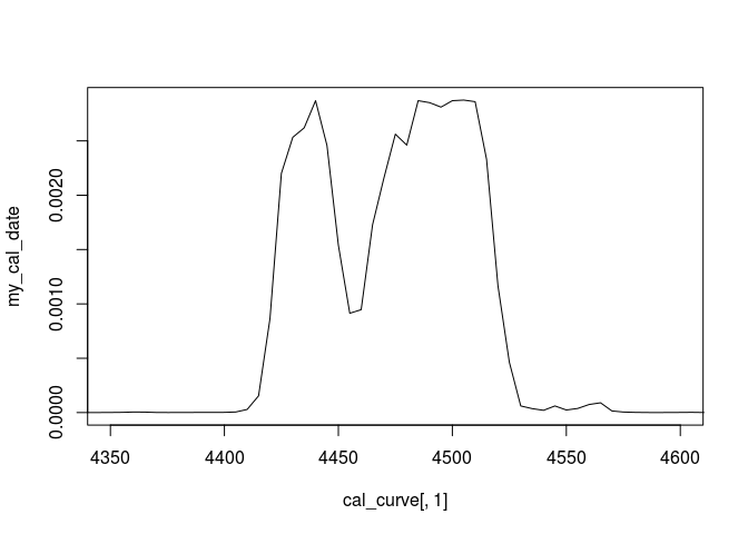
plot(cal_curve[,1],my_cal_date,type="l",xlim=c(4350,4600))
Got it? Fine! If not, continue reading…
Getting the Calibration Curve
For calibration we need two things: A date and the calibration curve.
Starting with the latter, you can obtain it at Radiocarbon. You can download it or access it directly from inside R, like I did in the upper code snippet. I will now go for the first alternative.
If you have downloaded it, you may like to inspect the file. It is
essentially a csv file, with a header spanning 11 rows. To load it into
your R, you can use the read.csv function, with skipping the first 11
rows, like this:
cal_curve <- read.csv("/path/to/your/calcurve",
                      skip=11,
                      header = F)
The data set contains several columns that are named in the header in a style not very conveniently for R users. We therefor name the columns manually:
colnames(cal_curve) <- c("CAL BP",
                         "14C age",
                         "Error",
                         "Delta 14C",
                         "Sigma")
Having the first component at hand, we proceed to arranging a date.
Making a date
What follows will be very simple: A 14C date consists of two components, a BP (before present in 14C years) and a standard deviation of the measurement. I will make a simple vector reflecting this structure, and since I am overly enthusiastic, I will also name the vector.
my_date <- c(4000, 25)
names(my_date) <- c("bp", "std")
Transforming the ‘curve’ to a matrix
Probably one of the most easy ways to calibrate a date is to use the calibration curve as transformation matrix. In the curve file we have information on the calibrated bp dates, the related 14C age and the error in years. Each of these value groups can be understood as probability distribution. Eg. for:
cal_curve[4500,]

##      CAL BP 14C age Error Delta 14C Sigma
## 4500   3205    3002    10      14.1   1.3
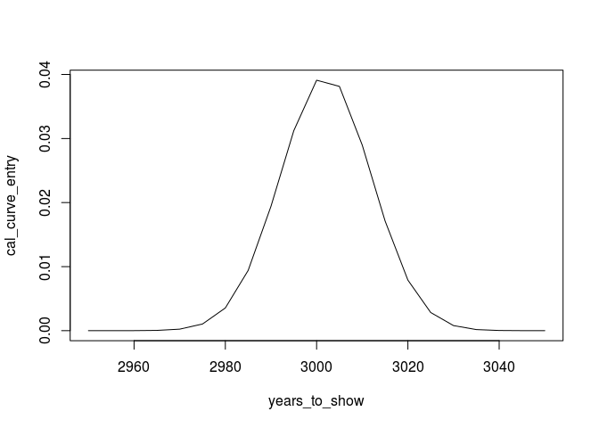
the calibrated bp year of 3205 results from a 14C age of 3002 with an error of 10, or from a normal distribution with a mean of 3002 and a standard deviation of 10 years:
years_to_show <- seq(2950,3050,by=5)
cal_curve_entry<-dnorm(years_to_show,3002,10)
plot(years_to_show,cal_curve_entry, type="l")
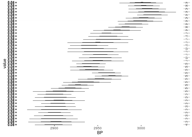
We can proceed with other dates (note: the libraries are only included to enhance the plot):
library(reshape2)
library(ggplot2)

years_to_show <- seq(2800,3050,by=5)
cal_curve_range <- cal_curve[4500:4540,]
cal_curve_entry_range <- apply(cal_curve_range,
                               1,
                               function(x) {
                                 dnorm(years_to_show,x[2],x[3])
                                 }
                               )
rownames(cal_curve_entry_range)<-years_to_show
cal_curve_entry_range[cal_curve_entry_range<1e-3]<-NA
dates_for_ggplot<-melt(t(cal_curve_entry_range))

m <- ggplot(dates_for_ggplot,aes(x=Var2,y=value,group=Var1))
graph <- m +
         geom_area() +
         facet_grid(Var1 ~ .) +
         scale_x_continuous("BP")
show(graph)

## Warning: Removed 1540 rows containing missing values (position_stack).
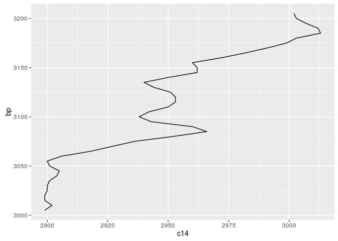
Compare the calibration curve for the respective time window:
cal_curve_for_ggplot<-data.frame(bp=cal_curve_range[,1],
                                 c14=cal_curve_range[,2])

m <- ggplot(cal_curve_for_ggplot,aes(x=bp,y=c14))
graph <- m + geom_line() + coord_flip()
show(graph)
The message of this is: The calibration curve can be expressed as matrix of probabilities, mapping one 14C year to one calendric BP year. Such a matrix can be constructed like that:
years <- cal_curve[,'CAL BP']

cal_matrix <- sapply(years,function(x) {
  dnorm(x,mean = cal_curve[,'14C age'],sd = cal_curve[,'Error'])
  })

rownames(cal_matrix)<-colnames(cal_matrix)<-years
Calibration by using the calibration curve as transformation matrix
This matrix we just created can be used to transform a vector of probabilities to a calibrated vector of probabilities. We have our date:
my_date

##   bp  std
## 4000   25
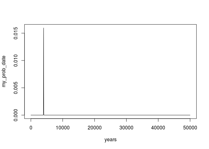
which represents a normal distributed density function with mean bp and standard deviation std. This can be expressed, with our years vector, as:
my_prob_date <- dnorm(years,
                      mean = my_date['bp'],
                      sd = my_date['std'])
plot(years,my_prob_date,type = 'l')
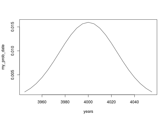
or if we zoom in to only the relevant parts
my_prob_date.window <- cbind(years,my_prob_date)
my_prob_date.window <- my_prob_date.window[my_prob_date.window[,2] > 1e-3,]
plot(my_prob_date.window,type = 'l')
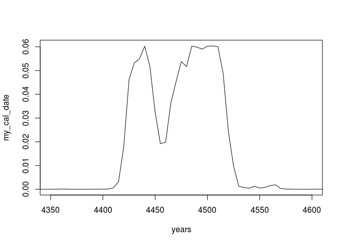
Now we can just multiply our vector with the transformation matrix to get a calibrated result:
my_cal_date <- as.vector(cal_matrix %*% my_prob_date)
# normalize, so that it sums up to 1
my_cal_date <- my_cal_date / sum(my_cal_date)
plot(years, my_cal_date, type = 'l', xlim=c(4350,4600))
Compare this to a ´Bchron´ calibration:
library(Bchron)

## Loading required package: inline

plot(
  Bchron::BchronCalibrate(4000,
                          25,
                          calCurves = 'intcal13'),
  xlim=c(4350,4600)
)
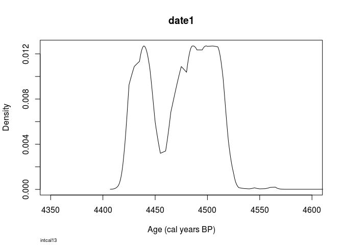
Looks pretty similar, doesn’t it?
Remember: it are essentially 4 steps in total to come from a date to a calibrated one, it is not rocket science. And 1 of them represents getting the curve, two other reshaping the calibration curve and the date, while only in one step you can do the calibration itself. Simple, isn’t it?