14C Calibration with JAGS
Intro
In this post I would like to continue what I have published already 4 years ago. This time I want to show how to calibrate a ¹⁴C-date using well-known Bayesian tools, specifically JAGS. JAGS stands for Just Another Gibbs Sampler, and is a program for analysing ‘Bayesian hierarchical models using Markov Chain Monte Carlo (MCMC) simulation’. This makes it clearly overqualified for our simple task, but it nicely shows a different perspective on the problem and also makes obvious the possibilities of how to extend this task even further.
Formulation of the problem
In the last post, I realised the bottom-up procedure and wrote an MCMC algorithm and a Gibbs sampler from scratch, or rather explained the method for doing so. Using the example of estimating pi, I showed how an MC method can be used to estimate unknown quantities that cannot be determined analytically. Based on this, I transferred the whole approach to radiocarbon calibration.
Prior
We can therefore dispense with all this here; we start by defining the problem from the other side. I had explained that (apart from technical things like the loop and a variable for collecting results) we need above all a prior and a likelihood function. The prior has not been explicitly specified by us, but it is implicit: Some calendar date, where all calendar dates per se have the same probability. This remains the same. However, for technical reasons, because we can only perform a calibration within the calibration curve, we have to restrict our prior somewhat: we can perform up to a maximum of the range of the calibration curve, which currently goes back to 55000 BP.
This poses a problem mathematically for the basic justification of the correctness of the procedure, but not practically. We simply have to be aware that the procedure will not work correctly for older data (or data that touches this fringe).
In formulaic language, we can express this prior as follows:
\[calDate ∼ U(0,55000)\]We pretend to know nothing per se about the possible temporal position of the calibrated date. This is not true, of course, we have the calibration curve and we will use it later to set the starting values for our analysis. But this is how we indicate the objectively available knowledge about it, namely that the calibrated date should be somewhere between today and the beginning of the calibration curve.
Likelihood
Next, let’s look at the definition of the likelihood of our calibrated date. Last time I expressed it like this:
likelihood <- function(proposal){dnorm(calf(proposal),bp,std)}
This is R-code, which says that the probability of a proposal is determined by how well the recalibrated 14C age (i.e. not calendar years) fits the measured value, which we have present. We randomly made suggestions from the whole range of the prior, and then looked to see how plausible this calendar year is, given our measurement. This has a normal distribution around the BP value with a certain standard deviation, which results from the measurement and the measurement inaccuracies.
The function calf() was a little help here, making a linear
approximation for the area between two calendar dates occupied in the
calibration curve. The R code was as follows:
calf<-approxfun(intcal13[,1],intcal13[,2])
Intuitively, this is what happens:
We have given two points. Between these we can determine the slope. If we now want to estimate another point for which the x-value lies between these points, we assume that it will behave in exactly the same way as the process we know through the two points and interpolate the y-value of the estimated point accordingly by sticking to these first two points.
The likelihood therefore consists of two elements: the normal distribution around the measured value, and the back-calibration of the estimated value, which we create using the linear approximation of the measured values of the calibration curve. In the first step, we assume for simplicity that the calibration curve is only a line and not a probability band. But we will incorporate this fact again later.
Let’s write it down roughly, then it could look like this:
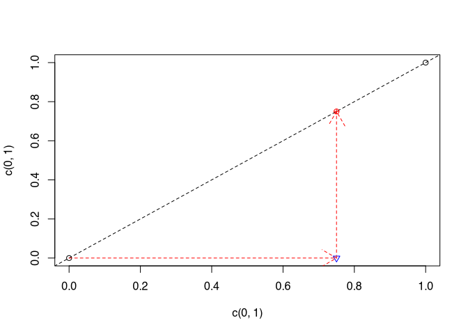
\[uncalDate = linearApproximation(calDate, CalibrationCurveBP_{uncal},CalibrationCurveBP_{cal}) \\ uncalDate \sim N(MeasurementBP, MeasurementSigma)\]Let’s take a look at the following illustration:
It does not matter whether I determine from the probability of the (red) recalibrated proposal with respect to the normal distribution of the measured value, or from the (black) measured value the probability with respect to the normal distribution around the recalibrated proposal: the result will be the same. Therefore, in the last line we can swap our uncalibrated proposal date with the measurement without changing anything in the probabilities:
\[MeasurementBP \sim N(uncalDate, MeasurementSigma)\]This gives us everything we need for a Bayesian model using JAGS, the prior and the likelihood. The programme takes care of all the other technical details. In return, however, we have to work some magic to persuade JAGS to cooperate. Before we get to that, let’s briefly write up the inside of our model:
\[calDate \sim U(0,55000)\\ \hspace{-2em}\\ uncalDate = linearApproximation(calDate, CalibrationCurveBP_{uncal},CalibrationCurveBP_{cal}) \\ MeasurementBP \sim N(uncalDate, MeasurementSigma)\]Putting JAGS to work
There are several packages for R to persuade JAGS to cooperate. The prerequisite, however, is that JAGS is installed at all on the operating system level. I will not discuss how to do this, as there are already too many operating systems to consider. But you can find your way around quite well via the project page and the internet help, I hope.
Rather, I would like to outline the R side of the task a little more closely.
We will use the package rjags, which is developed by Martyn Plummer,
who is also behind JAGS itself. This has to be installed (I have
commented it out for myself, for the first time the part behind the hash
has to be executed):
# install.packages("rjags")
And then be loaded
require(rjags)
## Loading required package: rjags

## Loading required package: coda

## Linked to JAGS 4.3.0

## Loaded modules: basemod,bugs
This puts the power of the programme at our disposal. In order to achieve a result quickly, I will put the simplest possible use at the beginning, we will also specify this in more detail later. So let’s turn to the implementation of our model in JAGS code. You remember the model from above, don’t you?
\[calDate \sim U(0,55000)\\ \hspace{-2em}\\ uncalDate = linearApproximation(calDate, CalibrationCurveBP_{uncal},CalibrationCurveBP_{cal}) \\ MeasurementBP \sim N(uncalDate, MeasurementSigma)\]First to the prior. We express this uniform distribution in JAGS language as follows:
# Prior
calDate ~ dunif(0,55000);
Here, dunif stands for the uniform distribution, the values given
behind it for the limits of the uniform distribution. That was easy. Now
for the likelihood. This consisted of two parts, the normal distribution
around the uncalibrated date and the recalibration of our proposal to
obtain this uncalibrated date. For this we want to use a linear
approximation. Fortunately, there is a function in JAGS that looks
pretty much like our formulaic proposal.
uncalDate <- interp.lin(calDate,calBP,C14BP);
Here are two variables (calBP, C14BP) that we have not yet added. This represents the calibrated and the uncalibrated values of the calibration curve, and we will give these values to the model as data (or better as constants) later.
Regarding the normal distribution, there is one small thing to note: JAGS, for historical reasons, does not expect the standard deviation as a parameter, but something called precision (and commonly abbreviated as τ or tau). This is nothing other than the inverse of the variance, or in terms of the standard deviation:
\[\tau = \frac{1}{\sigma^2}\]We have to add this small conversion to the model of the likelihood so that JAGS then understands it correctly. Therefore, the whole block for the normal distribution looks like this:
MeasurementBP ~ dnorm(uncalDate, tau)

tau <- 1/(pow(sigma,2)
With this we have the whole naive model (it does not yet take into account the standard deviation of the calibration curve itself) together:
# Prior
calDate ~ dunif(0,55000);

# Likelihood
uncalDate <- interp.lin(calDate,calBP,C14BP);

MeasurementBP ~ dnorm(uncalDate, tau)
tau <- 1/(pow(sigma,2)
By the way, the order does not matter, the main thing is that all elements are named and specified correctly. In order to make this usable for JAGS, we still have to transfer it into a variable and within it mark the actual model as a model by placing it in curly brackets with the word ‘model’ in front of it:
calibration_model <- "
  model{
    # Prior
    calDate ~ dunif(0,55000)

    # Likelihood
    uncalDate <- interp.lin(calDate,calBP,C14BP)

    MeasurementBP ~ dnorm(uncalDate, tau)
    tau <- 1/pow(sigma,2)
  }
"
The indentations are just for us to make it easier to read.
Wonderful, the model is ready, now we need the data. Firstly, there is the calibration curve. We want to take IntCal20, which is the latest version at the time of writing. We can download this from the net:
CalCurve <- read.csv(
  url("http://intcal.org/curves/intcal20.14c"),
  header=F, skip = 11)
colnames(CalCurve) <- c("calBP", "C14BP", "Sigma", "Delta_14C", "Sigma_Delta")
Furthermore, we need our measurement and its standard deviation. Let’s take a nice dating from the Neolithic:
MeasurementBP <- 5640
sigma <- 31
JAGS (or rjags) expects our data as a list, let’s put it together. A
small insertion nevertheless: interp.lin expects the values in ascending
order, the calibration curve delivers them in descending order. We have
to reverse this quickly using the R command rev():
data <- list(
  MeasurementBP = MeasurementBP,
  sigma = sigma,
  calBP = rev(CalCurve$calBP),
  C14BP = rev(CalCurve$C14BP)
)
With this we are basically done (we are not, we will see in a moment). To run jags now, we initialise the model:
m_init <- jags.model(textConnection(calibration_model), data=data)
## Compiling model graph
##    Resolving undeclared variables
##    Allocating nodes
## Graph information:
##    Observed stochastic nodes: 1
##    Unobserved stochastic nodes: 1
##    Total graph size: 19014
##
## Initializing model
Voila, we have an initialised model. Now, similar to our example by
hand, we can start the MCMC algorithm and have samples drawn. To do
this, we use the command coda.samples and specify from which variable
we want to get them, namely from calDate, as well as the number. Let’s
stay with 10000, as in the example by hand:
samples <- coda.samples(m_init, c('calDate'), 10000)
If we now have a summary of the sampled values, it is a rather unconvincing surprise:
summary(samples)
##
## Iterations = 1001:11000
## Thinning interval = 1
## Number of chains = 1
## Sample size per chain = 10000
##
## 1. Empirical mean and standard deviation for each variable,
##    plus standard error of the mean:
##
##           Mean             SD       Naive SE Time-series SE
##      2.678e+04      7.064e-01      7.064e-03      1.056e-02
##
## 2. Quantiles for each variable:
##
##  2.5%   25%   50%   75% 97.5%
## 26779 26780 26780 26781 26782
All samples, with few deviations, took place around the year 26780. We expected that to be better. This can also be better if we let the algorithm start at the right place.
Another way to see that something is going wrong here is to have the sampling process itself displayed graphically. To do this, you can simply apply the plot command to the result of the sampling:
plot(samples)
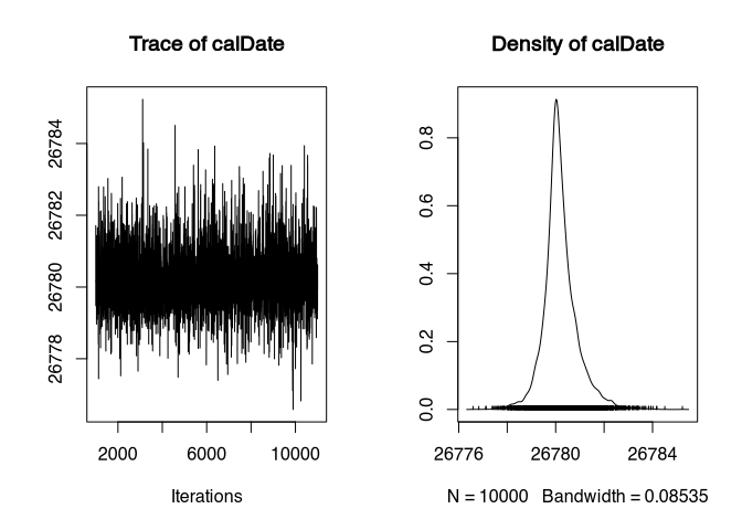
On the left we see the so-called trace plot. Generally, this should look like “a hairy caterpillar”. Which it does here. However, the values only jump back and forth between 26784 and 26778. The density plot on the right also looks quite wrong, with a very pronounced peak and a steep slope on both sides. This is not how a calibrated datum should look!
We do not specify a frame within which the date can lie, but very small probabilities over the entire span of the 50,000 years mean that the algorithm cannot navigate reasonably along the suggestions, and therefore always remains at the starting point. Therefore, we roughly estimate the position of the calibrated date on the basis of the calibration curve:
naive_cal <- approx(CalCurve$C14BP, CalCurve$calBP, data$MeasurementBP)$y
## Warning in regularize.values(x, y, ties, missing(ties), na.rm = na.rm):
## collapsing to unique 'x' values
There is the linear approximation again, but this time in reverse. We estimate the calibrated date from the uncalibrated date. Of course, this is not allowed for a real calibration, but it gives us a good starting point to run through the whole probability range of the calibration. Accordingly, we get a warning that several places would fit, and only one is selected. However, this is sufficient as a starting value, which we give via another variable (which I call inits):
inits <- list(calDate = naive_cal)
m_init <- jags.model(textConnection(calibration_model), data=data, inits = inits)
## Compiling model graph
##    Resolving undeclared variables
##    Allocating nodes
## Graph information:
##    Observed stochastic nodes: 1
##    Unobserved stochastic nodes: 1
##    Total graph size: 19014
##
## Initializing model
samples <- coda.samples(m_init, c('calDate'), 10000)
summary(samples)
##
## Iterations = 1001:11000
## Thinning interval = 1
## Number of chains = 1
## Sample size per chain = 10000
##
## 1. Empirical mean and standard deviation for each variable,
##    plus standard error of the mean:
##
##           Mean             SD       Naive SE Time-series SE
##      6417.5136        39.6977         0.3970         0.9805
##
## 2. Quantiles for each variable:
##
##  2.5%   25%   50%   75% 97.5%
##  6325  6401  6423  6441  6484
That is already more credible! The calibrated results range between 6325 and 6484 with a 95% confidence interval. Let’s look at the plot of the samples:
plot(samples)
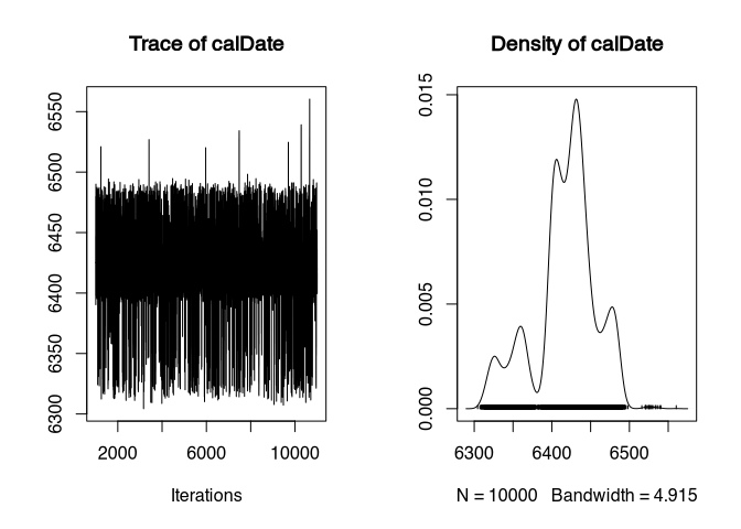
That’s better. The “caterpillar” has more legs than hair - less deviation into the lower than into the higher range, but the density plot is already far more credible.
And then compare the result with a calibration using another method, e.g. rcarbon:
if (!require(rcarbon)) install.packages("rcarbon") # Install, if not already present
## Loading required package: rcarbon
require(rcarbon) # Load in any case
rcarbon_result <- calibrate(data$MeasurementBP, data$sigma)
## [1] "Calibrating radiocarbon ages..."
##   |                                                                              |                                                                      |   0%  |                                                                              |======================================================================| 100%[1] "Done."
plot(rcarbon_result)
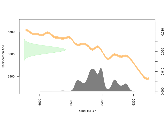
The similarities are clearly visible!
Now there is one more thing we have not taken into account: The calibration curve itself also has a range of uncertainty, as is clear from the data from IntCal20 itself:
´
head(CalCurve)
##   calBP C14BP Sigma Delta_14C Sigma_Delta
## 1 55000 50100  1024     528.5       193.9
## 2 54980 50081  1018     528.3       192.7
## 3 54960 50063  1013     527.9       191.7
## 4 54940 50043  1007     527.8       190.6
## 5 54920 50027  1003     527.0       189.5
## 6 54900 50009   997     526.6       188.4
It clearly says sigma! However, this is not a problem, we can interpolate this sigma for each proposed date as well and then insert it into the variation range of the normal distribution just like the sigma of the measurement itself:
better_calibration_model <- "
  model{
    # Prior
    calDate ~ dunif(0,55000)

    # Likelihood
    uncalDate <- interp.lin(calDate,calBP,C14BP)
    sigmaCalCurve <- interp.lin(calDate,calBP,C14Sigma) # Here we now interpolate the Uncertainity of the CalCurve itself

    MeasurementBP ~ dnorm(uncalDate, tau)

    tau <- 1/(pow(sigma,2)+pow(sigmaCalCurve,2)) # Here comes the CalCurve uncertainity into the Model
  }
"
We need to add the source for the uncertainity to the data
data$C14Sigma <- CalCurve$Sigma
And now we do the same as before:
m_init <- jags.model(textConnection(better_calibration_model), data=data, inits = inits)
## Compiling model graph
##    Resolving undeclared variables
##    Allocating nodes
## Graph information:
##    Observed stochastic nodes: 1
##    Unobserved stochastic nodes: 1
##    Total graph size: 28519
##
## Initializing model
samples_better <- coda.samples(m_init, c('calDate'), 10000)
Let’s have a look at the summary of the samples:
summary(samples_better)
##
## Iterations = 1001:11000
## Thinning interval = 1
## Number of chains = 1
## Sample size per chain = 10000
##
## 1. Empirical mean and standard deviation for each variable,
##    plus standard error of the mean:
##
##           Mean             SD       Naive SE Time-series SE
##      6413.7099        45.2159         0.4522         0.9311
##
## 2. Quantiles for each variable:
##
##  2.5%   25%   50%   75% 97.5%
##  6321  6393  6420  6443  6486
And compare that with the previous run:
summary(samples)
##
## Iterations = 1001:11000
## Thinning interval = 1
## Number of chains = 1
## Sample size per chain = 10000
##
## 1. Empirical mean and standard deviation for each variable,
##    plus standard error of the mean:
##
##           Mean             SD       Naive SE Time-series SE
##      6417.5136        39.6977         0.3970         0.9805
##
## 2. Quantiles for each variable:
##
##  2.5%   25%   50%   75% 97.5%
##  6325  6401  6423  6441  6484
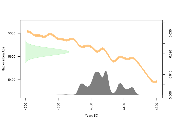
Actually, not that much has changed. Let’s plot this over the date calibrated by rcarbon:
plot(rcarbon_result$grids$`1`$calBP, rcarbon_result$grids$`1`$PrDens, type = "l")
lines(density(samples[[1]]), col="red")
lines(density(samples_better[[1]]), col="green")
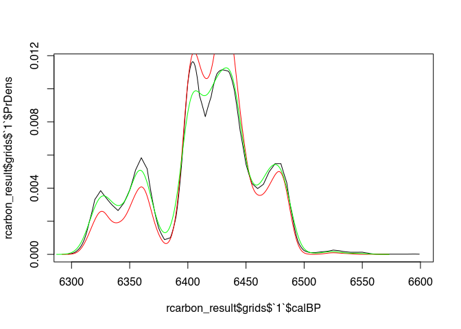
Especially in the marginal areas, the green curve (our samples_better) should provide more reliable results.
Convergence
Now we go one step further. We have arbitrarily set 10000 repetitions for our result. But is that enough? Or too much? And is the result reliable? There is a way to estimate this by running several estimates in parallel. If all of them come to the same result, then this should also be consistent.
To do this, we simply specify that more than one chain is to be computed. To illustrate the effect, I shorten the adaptation time of the model, which is set to 1000 iterations by default and ensures that the sampler works more effectively. I also set the start value for one of the chains to something less optimal:
diff_inits <- list(inits,
                   list( calDate = inits$calDate + 300))

m_init <- jags.model(textConnection(better_calibration_model),
                     data=data,
                     inits = diff_inits,
                     n.chains = 2, # two chains
                     n.adapt=50
                    )
## Compiling model graph
##    Resolving undeclared variables
##    Allocating nodes
## Graph information:
##    Observed stochastic nodes: 1
##    Unobserved stochastic nodes: 1
##    Total graph size: 28519
##
## Initializing model

## Warning in jags.model(textConnection(better_calibration_model), data = data, :
## Adaptation incomplete
samples_better <- coda.samples(model = m_init,
                               variable.names = c('calDate'),
                               n.iter = 10000)
## NOTE: Stopping adaptation
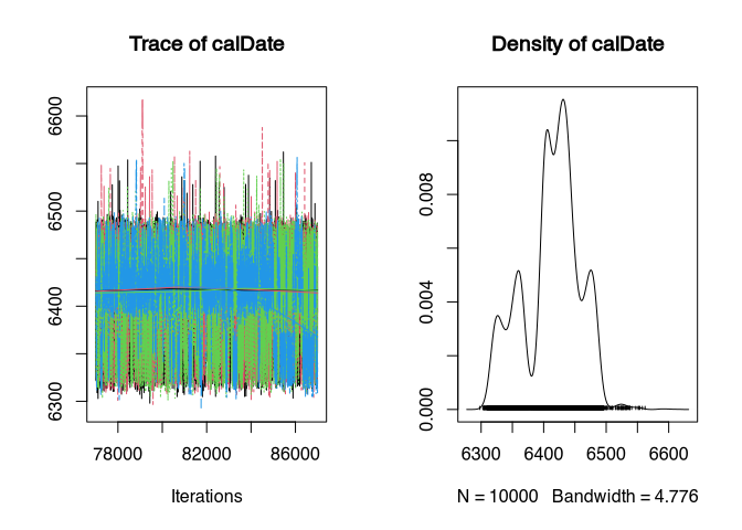
plot(samples_better)
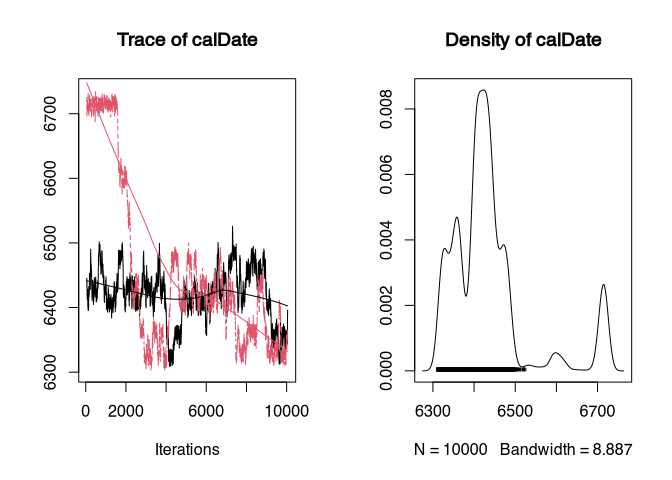
The first chain is rendered in black, the second in red. We can see that the chains differ from each other. It takes time for them to sample in the same area. This is called that they “converge”. Accordingly, only after a certain point in time do the samples make sense. To determine this, one could perhaps read it from the trace plot. However, it is better to use the generally recognised statistic for this, the Brooks-Gelman-Rubin (BGR) statistic.
gelman.diag(samples_better)
## Potential scale reduction factors:
##
##         Point est. Upper C.I.
## calDate       1.22       1.75
This value should be close to 1, then we have achieved convergence. Generally, it is said that it should not exceed 1.1. Here it is higher. This is due to the different starting values, but also because our sampler does not work optimally due to lack of adaptation. We can also take a graphical look at the point at which convergence could be achieved:
gelman.plot(samples_better)
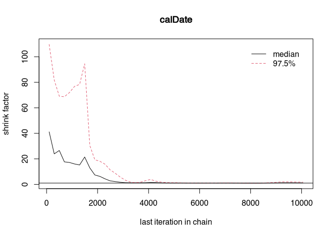
At a certain point, both curves may run close to zero. That would be the point at which convergence would be reached. What we can do (we have deliberately made the sampler worse) is to let the chains run longer and throw away the first part. We know that at the beginning of the run of the MCMC, the samples are taken from not very probable areas. It is good practice in Bayesian modelling to ignore the first results. This is also called the burn-in phase.
To make the chains run longer, we can simply repeat the sampling process:
samples_better <- coda.samples(model = m_init,
                               variable.names = c('calDate'),
                               n.iter = 10000)
gelman.plot(samples_better)
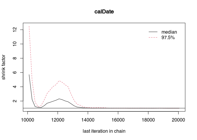
That should look better now. Perhaps even complete convergence has been achieved? Let’s have a look:
gelman.diag(samples_better)
## Potential scale reduction factors:
##
##         Point est. Upper C.I.
## calDate          1          1
You can continue this until you are satisfied with the Gelman-Rubin-Brooks statistics. You can try to optimise the time of the burn-in, as you do not want to sample the computer for an unnecessarily long time.
So, let’s end the whole thing with our model running according to the rules with 4 chains. Since the model can now fully adapt, there is no burn-in at all in this simple case. Therefore, I set extra false start values and used a while loop to first update with 2000 samples until the statistics are sufficient, and then I take the final 10000 samples.
extra_diff_inits <- list(
                   list( calDate = inits$calDate + 100),
                   list( calDate = inits$calDate + 200),
                   list( calDate = inits$calDate + 300),
                   list( calDate = inits$calDate + 385)
                   )

m_init <- jags.model(textConnection(better_calibration_model),
                     data=data,
                     inits = extra_diff_inits,
                     n.chains = 4
                    )
## Compiling model graph
##    Resolving undeclared variables
##    Allocating nodes
## Graph information:
##    Observed stochastic nodes: 1
##    Unobserved stochastic nodes: 1
##    Total graph size: 28519
##
## Initializing model
it <- 1 # I like to take count of the iteration, not necessary in real world

not_converged <- TRUE

while(not_converged){
samples_better <- coda.samples(model = m_init,
                               variable.names = c('calDate'),
                               n.iter = 2000)
it <- it + 1
not_converged <- gelman.diag(samples_better)$psrf[1,1]>1.1
}

samples_better <- coda.samples(model = m_init,
                               variable.names = c('calDate'),
                               n.iter = 10000)

plot(samples_better)
gelman.diag(samples_better)
## Potential scale reduction factors:
##
##         Point est. Upper C.I.
## calDate          1          1
It took 39 iterations before convergence was achieved. And now here is our calibrated date, where we may assume a successful convergence of 4 chains.
We can then display the result in a graphically appealing way. For this purpose, I will use the bayesplot package, but there are a large number of packages that can be used for this task.
if (!require(bayesplot)) install.packages("bayesplot") # Install, if not already present
## Loading required package: bayesplot

## This is bayesplot version 1.8.1

## - Online documentation and vignettes at mc-stan.org/bayesplot

## - bayesplot theme set to bayesplot::theme_default()

##    * Does _not_ affect other ggplot2 plots

##    * See ?bayesplot_theme_set for details on theme setting
require(bayesplot) # Load in any case
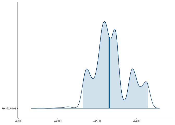
bayesplot::mcmc_areas(samples_better, prob = 0.95,
transformations = function(x) 1950 - x)
For comparison, the rcarbon version again:
plot(rcarbon_result, calendar = "BCAD")
So, by using JAGS, we learned how to set up and implement our model formulaically, and also how to test and improve its reliability. And it wasn’t that hard, was it?